Cool Applications of Linear Algebra

Linear Algebra has tons of Real world Applications which you may have never imagined or at least heard of. In this article, I have tried to explain two of them, particularly related to the Computer Vision Field and Robotic System Design Field since I love the two fields over any other field.
Computer Vision: Detecting Corners/Features of an Image
Related Concepts in Linear Algebra: Eigenvalues, Eigenvectors, Characteristic Polynomial, Quadratic Forms, Principal Axis Theorem, Orthogonal matrix, Diagonalization
Problem Identification
In computer vision field finding corners/features in an image(\(I(x, y)\)) is a key operation which is done prior to many advanced applications such as feature mapping, panorama stitching and 3D reconstruction. A corner can be identified as a point in an image whose neighborhood is locally unique to the given image. When comparing this neighborhood with any of the surrounding neighborhoods, significant difference can be observed between them.
This difference can be quantified mathematically using the following function evaluated over a region called a window(\(W\)). Here the most basic Error function is used to make the explanation easy, and this may vary in different implementation of corner detection algorithms.
\[E(u,v) = \sum_{(x,y) \in W}[I(x+u, y+v) – I(x, y)]^2\]
This function can be further simplified using Taylor series and can be rearranged to get an expression in the Quadratic form associated with \(M\) where the \(M\) is called the Second Moment Matrix which consists of summation of quadratic forms of gradients of the image over a window centered at the point of interest. Here gradient of the image along x axis is \(I_{x}\) while \(I_{y}\) is the gradient along y axis.
\[\begin{split} E(u,v) &= \sum_{(x,y) \in W}[I_{x}^{2}.u^{2}+2.I_{x}.I_{y}.u.v + I_{y}^{2}.v^{2}]\\ &= \begin{bmatrix} u & v \end{bmatrix} \begin{bmatrix} \sum_{(x,y) \in W}[I_x ^2 ]& \sum_{(x,y) \in W}[I_x I_y] \\ \sum_{(x,y) \in W}[I_x I_y]& \sum_{(x,y) \in W}[I_y ^2 ] \end{bmatrix} \begin{bmatrix} u \\ v \end{bmatrix}\\ &=\begin{bmatrix} u & v \end{bmatrix}M\begin{bmatrix} u \\ v \end{bmatrix}\\ E(\underline{x})&= \underline{x}^\top M \underline{x} \end{split} \label{euv}\]
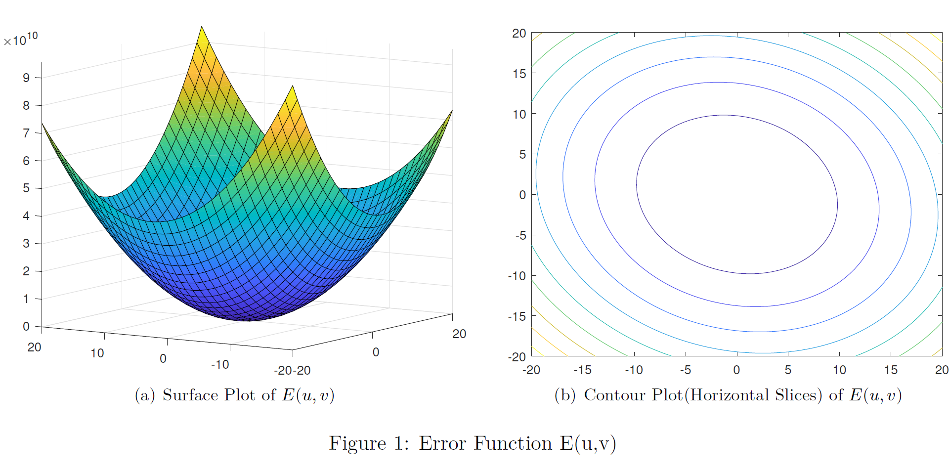
The plot of the above function looks like follows for a given point where the \(\sum_{(x,y) \in W}[I_x ^2 ]= 105983042.0\), \(\sum_{(x,y) \in W}[I_x I_y]=13718014.0\) and \(\sum_{(x,y) \in W}[I_y ^2 ]=105671174.0\). If the point of interest is a corner it will give a very large Error (\(E(u,v)\)) value even for a very low (\(u,v\)) shift in any direction. This can be intuitively recognized as a steep surface(more narrower bowl shape) as depicted in Figure 1 (a).
Solution through concepts of Linear Algebra
This narrowness can be mathematically quantified by examining a horizontal slice of the Surface plot. Consider one particular contour in Figure 1 (b) , then along that contour, function value is a constant i.e \(E(\underline{x}) = constant = \underline{x}^\top M \underline{x}\) and then the above Expression (\(E(u,v)\)) represents equation of an ellipse. If the surface is narrow, the radii of the ellipse must be small for a given \(E(u,v)\) value. That is function value must increase rapidly as we moves outward from the point of interest. Lengths of the major and minor axes(radii) of the ellipse are given by \(\lambda_{min}^{-\frac{1}{2}}\) and \(\lambda_{max}^{-\frac{1}{2}}\) respectively, where the \(\lambda_{min}\) and \(\lambda_{max}\) are the eigenvalues associated with the second moment matrix \(M\). We can prove this as follows.
Since \(M\) is a symmetric matrix, an Orthogonal(\(P^\top=P^{-1}\)) matrix \(P\) can be found such that \(\underline{x} = P\underline{y}\) which transforms \(E(\underline{x}) = \underline{x}^\top M \underline{x}\) into the form \(E(\underline{y}) = \underline{y}^\top D \underline{y}\) where \(D\) is a diagonal matrix consists of the eigenvalues of the \(M\). The columns of matrix \(P\) consists of the eigenvectors associated with the eigenvalues of the second moment matrix \(M\).
\[\begin{split} E(\underline{x}) &= \underline{x}^\top M \underline{x}\\ &= (P\underline{y})^\top M (P\underline{y})\\ &= (\underline{y}^\top P^\top) M (P\underline{y})\\ &= \underline{y}^\top (P^\top M P)\underline{y}\\ &= \underline{y}^\top D \underline{y}\\ E({y_{1},y_{2}})&= \begin{bmatrix} y_{1} & y_{2} \end{bmatrix} \begin{bmatrix} \lambda_{min} & 0 \\ 0 & \lambda_{max} \end{bmatrix} \begin{bmatrix} y_{1} \\ y_{2} \end{bmatrix}\\ \end{split} \label{orthdiag}\]
Comparing result of Expression (\(E({y_{1},y_{2}})\)) with the standard form of an ellipse,
\[\begin{split} {\frac{x^2}{a^2} + \frac{y^2}{b^2}} &= {\begin{bmatrix} x & y \end{bmatrix} \begin{bmatrix} 1/a^2 & 0 \\ 0 & 1/b^2 \end{bmatrix} \begin{bmatrix} x \\ y \end{bmatrix}} \\ &= {\begin{bmatrix} y_{1} & y_{2} \end{bmatrix} \begin{bmatrix}\lambda_{min} & 0 \\ 0 & \lambda_{max} \end{bmatrix} \begin{bmatrix} y_{1} \\ y_{2} \end{bmatrix}}\\ \end{split}\]
Therefore, \(1/a^2 = \lambda_{min}\) and \(1/b^2 = \lambda_{max}\). Which yields that \(a = \lambda_{min}^{-\frac{1}{2}}\) and \(b = \lambda_{max}^{-\frac{1}{2}}\).
Therefore to find corners in an image all we have to do is find the eigenvalues associated with each second moment matrix for each pixel\((x,y)\) in an image. According to the magnitudes of eigenvalues following classification can be done.
At a Corner: \(E(u,v)\) increases rapidly in any direction and therefore both eigenvalues are large.
At an Edge: \(E(u,v)\) increases rapidly only in one direction and therefore one eigenvalue is relatively larger than the other.
At a flat area: \(E(u,v)\) does not increase rapidly and therefore both eigenvalues are small.
Calculating eigenvalues is computationally expensive therefore what is known as Corner Response Function(R) is used when implementing algorithms. Here \(\alpha\) \(\in\) [0.04,0.06] and At a Corner: R \(\gg\) 0, At an Edge: R \(<\) 0, At a flat area: \(|R|\) is small. Therefore corners can be extracted by applying an appropriate threshold value for R.
\[\begin{split} R &= det(M) - \alpha* trace(M)^2\\ & = \lambda_{min}*\lambda_{max} - \alpha*(\lambda_{max} + \lambda_{min})^2 \end{split}\]
Robotic Systems: Coordinate frame Transformation
Related Concepts in Linear Algebra: Linear Transformations, Matrix Transformations, Change of basis, Matrix Multiplication
Problem Identification
When robot arms are used in industrial activities, robot engineer needs to make sure the end-effector(gripper or any other tool attached at the end of the arm) of the robot arm is at the exact location in the exact orientation at the operation. Otherwise the required behavior of the arm can not be obtained. Problem is usually robot takes the measurements using sensors or cameras placed somewhere else in the system and therefore these measurements(position vectors) are in with respect to those sensor’s or camera’s coordinate frame while the robot arm operates with respect to some other(Robot base) coordinate frame. Flowing figure illustrates this situation.
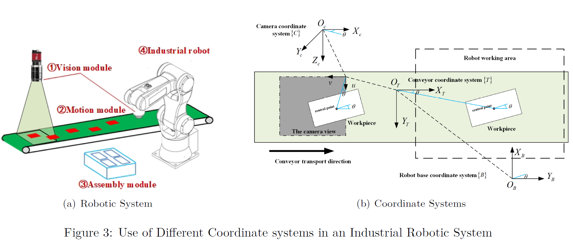
Therefore to make use of the information gathered by the sensors/cameras first we need to transform position vectors gathered by camera with respect to its coordinate frame, in to robot arm’s base coordinate frame. Then we can use inverse kinematics to calculate the required rotation angles and translations that we should provide to the arm to get the required behavior.
Solution through concepts of Linear Algebra
In order to fully describe an object in the 3D world we need its Rotation and Translation with respect to some reference(in this case the robot arm) coordinate frame(\(\alpha\)). For that the object of interest(in this case the sensor/camera) must be given its own coordinate frame(\(\beta\)) too. The mathematical way to represent differences between the reference frame and the object’s frame is called the Homogeneous Transformation Matrix in Robotics and it is denoted as,
\(H^{\alpha}_{\beta}\) : read as transformation of frame \(\beta\) with respect to the frame \(\alpha\)
This \(H^{\alpha}_{\beta}\) can be mathematically represented as a \(4 \times 4\) matrix which consists of \(3 \times 3\) Rotation matrix and a \(3 \times 1\) Translation matrix with last row as \([0~0~0~1]\) to make it \(4 \times 4\) square matrix to make the computation easy.
\[\begin{split} H^{\alpha}_{\beta} &= \begin{bmatrix} r_{11} & r_{12} & r_{13} & d_1 \\ r_{21} & r_{22} & r_{23} & d_2 \\ r_{31} & r_{32} & r_{33} & d_3 \\ 0 & 0 & 0 &1 \\ \end{bmatrix} \end{split}\]
There are 6 Principal Movements as, rotations about 3 axes(X,Y,Z) and translations along 3 axes(X,Y,Z). Correct combination(obtain by multiplying required principal matrices like \(Rot(e_i,\theta_m)*Trans(e_j,d_k)\)) of these 6 principal movements can be used to get any of the advanced transformations, from the reference frame to object’s frame. Those basic matrices are as follows where \(e_i\) refers to the elements in standard basis( \(e_1 = [1 ~0~ 0]^\top\), \(e_2 = [0 ~1~ 0]^\top\) and \(e_3 = [0 ~0~ 1]^\top\)) while \(\theta_i\) indicates how many degrees the object has rotated about the \(e_i\) basis vector. Additionally \(d_i\) indicates the displacement along the direction of \(e_i\) basis vector(axis).
| Principal Rotations about axes(X,Y,Z) | Principal Translations along axes(X,Y,Z) |
|---|---|
| \(Rot(e_1,\theta_1) = \begin{bmatrix} 1 & 0 & 0 & 0 \\ 0 & \cos(\theta_1) & -\sin(\theta_1) & 0 \\ 0 & \sin(\theta_1) & \cos(\theta_1) & 0 \\ 0 & 0 & 0 &1 \\ \end{bmatrix}\) | \(Trans(e_1,d_1)= \begin{bmatrix} 1 & 0 &0 & d_1 \\ 0 & 1 & 0 & 0 \\ 0 & 0 & 1 & 0 \\ 0 & 0 &0 & 1 \\ \end{bmatrix}\) |
| \(Rot(e_2,\theta_1) = \begin{bmatrix} \cos(\theta_1) & 0 & \sin(\theta_1) & 0 \\ 0 & 1 & 0 & 0 \\ -\sin(\theta_1) & 0 & \cos(\theta_1) & 0 \\ 0 & 0 & 0 &1 \\ \end{bmatrix}\) | \(Trans(e_2,d_2) = \begin{bmatrix} 1 & 0 &0 & 0 \\ 0 & 1 & 0 & d_2 \\ 0 & 0 & 1 & 0 \\ 0 & 0 & 0 & 1 \\ \end{bmatrix}\) |
| \(Rot(e_3,\theta_1) = \begin{bmatrix} \cos(\theta_1) & -\sin(\theta_1)&0 & 0 \\ \sin(\theta_1) & \cos(\theta_1) &0 & 0 \\ 0&0 &1 & 0 \\ 0 & 0 & 0 &1 \\ \end{bmatrix}\) | \(Trans(e_3,d_3) = \begin{bmatrix} 1 & 0 &0 & 0 \\ 0 & 1 & 0 & 0 \\ 0 & 0 & 1 & d_3 \\ 0 & 0 & 0 & 1 \\ \end{bmatrix}\) |
Once we construct the Homogeneous Transformation Matrix which transforms robot base frame into camera frame, we just have to multiply the position vectors obtained w.r.t camera frame by this transformation matrix to get the corresponding position vectors in the robot base frame. Let \(^1u = [u_1 ~u_2~ u_3~1]^\top\) be a position vector(homogeneous) of an object in the camera frame and \(H^{0}_{1}\) be the homogeneous transformation matrix, then the position vector of the object in the robot base frame is, say \(^0u\)
\[\begin{split} ^0u &= H^{0}_{1}* ^1u\\ ^0u &= {\begin{bmatrix} r_{11} & r_{12} & r_{13} & d_1 \\ r_{21} & r_{22} & r_{23} & d_2 \\ r_{31} & r_{32} & r_{33} & d_3 \\ 0 & 0 & 0 &1 \\ \end{bmatrix}} * \begin{bmatrix} u_1 \\u_2\\ u_3\\1 \end{bmatrix} \end{split}\]
Moreover, since the Homogeneous Transformation Matrix is invertible, following expression is also valid which makes it possible to move between coordinate systems easily. \[{H^{0}_{1}}^{-1} = H^{1}_{0}\]
That’s It. Hope you get some idea about the applications of this awesome branch of mathematics and now you may feel why you need to have a clear understanding about these concepts in mathematics. I have mentioned the related references so you can go through them to get a better understanding. Moreover If you need the pdf version of this article, it can be found here and all the source codes(LaTeX and MatLab) used to produce the document can be found here.
- Harris Corner Detection (Full Explanation)
- Bimalka Thalagala. bimalka98/Computer-Vision-and-Image-Processing
- Robotics 1 kinematics (rotation matrices) - YouTube.
- Robotics: Transformation Matrices - Part 1,2,3 - YouTube.
- A Robotic Automatic Assembly System Based on Vision
Feel free to comment your ideas and point out mistakes if I have done any, when writing this article.